ランダムフォレスト
Contents
ランダムフォレスト
ランダムフォレストについては以下を参照してください。 https://scikit-learn.org/stable/modules/ensemble.html#forest
データとモジュールのロード
学習に使うデータをロードします。
import pandas as pd
from sklearn import model_selection

data = pd.read_csv("input/pn_same_judge_preprocessed.csv")
train, test = model_selection.train_test_split(data, test_size=0.1, random_state=0)
from sklearn.pipeline import Pipeline
from sklearn.feature_extraction.text import TfidfVectorizer
from sklearn.metrics import PrecisionRecallDisplay
決定木
ランダムフォレストは決定木の バギング によりアンサンブル学習する手法なので、 まずは決定木から始めましょう。
決定木を学習するには
sklearn.tree.DecisionTreeClassifier
を使います。
ここでは正則化のために max_depth, min_samples_leaf パラメータを指定しています。
from sklearn.tree import DecisionTreeClassifier
pipe_dt = Pipeline([
    ("vect", TfidfVectorizer(tokenizer=str.split)),
    ("clf", DecisionTreeClassifier(max_depth=2, min_samples_leaf=10, random_state=0)),
])
pipe_dt.fit(train["tokens"], train["label_num"])
Pipeline(steps=[('vect',
                 TfidfVectorizer(tokenizer=<method 'split' of 'str' objects>)),
                ('clf',
                 DecisionTreeClassifier(max_depth=2, min_samples_leaf=10,
                                        random_state=0))])
In a Jupyter environment, please rerun this cell to show the HTML representation or trust the notebook. On GitHub, the HTML representation is unable to render, please try loading this page with nbviewer.org.
Pipeline(steps=[('vect',
                 TfidfVectorizer(tokenizer=<method 'split' of 'str' objects>)),
                ('clf',
                 DecisionTreeClassifier(max_depth=2, min_samples_leaf=10,
random_state=0))])TfidfVectorizer(tokenizer=<method 'split' of 'str' objects>)
DecisionTreeClassifier(max_depth=2, min_samples_leaf=10, random_state=0)
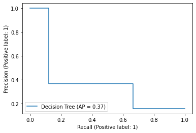
score_dt = pipe_dt.predict_proba(test["tokens"])[:,1]
PrecisionRecallDisplay.from_predictions(
    y_true=test["label_num"],
    y_pred=score_dt,
    name="Decision Tree",
)
<sklearn.metrics._plot.precision_recall_curve.PrecisionRecallDisplay at 0x7f0f7578eeb0>
木を表示してみましょう。
import matplotlib.pyplot as plt
from sklearn.tree import plot_tree

plot_tree(pipe_dt["clf"], filled=True)
plt.show()
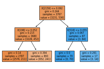
words = pipe_dt["vect"].get_feature_names_out()
words[2159], words[198], words[518]
('残念', 'が', 'ます')
ランダムフォレスト
ランダムフォレストは決定木をバギングしたモデルです。
sklearn.ensemble.BaggingClassifier を使うと次のように実装できます。
from sklearn.ensemble import BaggingClassifier
bagging = BaggingClassifier(
    DecisionTreeClassifier(splitter="random"),  # splitterはrandomに設定して、特徴量をランダムに探索する
    n_estimators=1000,
    random_state=0,
    n_jobs=-1,  # 全てのCPUを使う
)
pipe_bagging = Pipeline([
    ("vect", TfidfVectorizer(tokenizer=str.split)),
    ("clf", bagging),
])
pipe_bagging.fit(train["tokens"], train["label_num"])
Pipeline(steps=[('vect',
                 TfidfVectorizer(tokenizer=<method 'split' of 'str' objects>)),
                ('clf',
                 BaggingClassifier(base_estimator=DecisionTreeClassifier(splitter='random'),
                                   n_estimators=1000, n_jobs=-1,
                                   random_state=0))])
In a Jupyter environment, please rerun this cell to show the HTML representation or trust the notebook. On GitHub, the HTML representation is unable to render, please try loading this page with nbviewer.org.
Pipeline(steps=[('vect',
                 TfidfVectorizer(tokenizer=<method 'split' of 'str' objects>)),
                ('clf',
                 BaggingClassifier(base_estimator=DecisionTreeClassifier(splitter='random'),
                                   n_estimators=1000, n_jobs=-1,
random_state=0))])TfidfVectorizer(tokenizer=<method 'split' of 'str' objects>)
BaggingClassifier(base_estimator=DecisionTreeClassifier(splitter='random'),
n_estimators=1000, n_jobs=-1, random_state=0)DecisionTreeClassifier(splitter='random')
DecisionTreeClassifier(splitter='random')
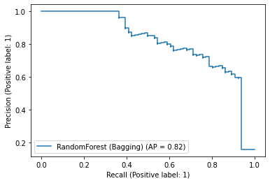
score_bagging = pipe_bagging.predict_proba(test["tokens"])[:,1]
PrecisionRecallDisplay.from_predictions(
    y_true=test["label_num"],
    y_pred=score_bagging,
    name="RandomForest (Bagging)",
)
<sklearn.metrics._plot.precision_recall_curve.PrecisionRecallDisplay at 0x7f0f7167f460>
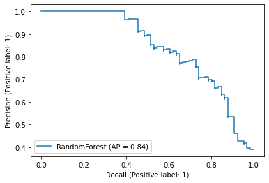
BuggingClassifier を使って実装しなくても、scikit-learn は sklearn.ensembleRandomForestClassifier を提供しています。 ランダムフォレストを使う場合は、こちらを使う方がいいでしょう。
from sklearn.ensemble import RandomForestClassifier
random_forest = RandomForestClassifier(
    n_estimators=1000,
    random_state=0,
    n_jobs=-1,
)
pipe_rf = Pipeline([
    ("vect", TfidfVectorizer(tokenizer=str.split)),
    ("clf", random_forest),
])
pipe_rf.fit(train["tokens"], train["label_num"])
Pipeline(steps=[('vect',
                 TfidfVectorizer(tokenizer=<method 'split' of 'str' objects>)),
                ('clf',
                 RandomForestClassifier(n_estimators=1000, n_jobs=-1,
                                        random_state=0))])
In a Jupyter environment, please rerun this cell to show the HTML representation or trust the notebook. On GitHub, the HTML representation is unable to render, please try loading this page with nbviewer.org.
Pipeline(steps=[('vect',
                 TfidfVectorizer(tokenizer=<method 'split' of 'str' objects>)),
                ('clf',
                 RandomForestClassifier(n_estimators=1000, n_jobs=-1,
random_state=0))])TfidfVectorizer(tokenizer=<method 'split' of 'str' objects>)
RandomForestClassifier(n_estimators=1000, n_jobs=-1, random_state=0)
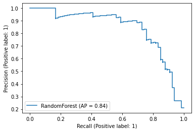
score_rf = pipe_rf.predict_proba(test["tokens"])[:,1]
PrecisionRecallDisplay.from_predictions(
    y_true=test["label_num"],
    y_pred=score_rf,
    name="RandomForest",
)
<sklearn.metrics._plot.precision_recall_curve.PrecisionRecallDisplay at 0x7f0f71087400>
特徴量の重要度
ランダムフォレストでは、 feature_importances_ 属性を見ることで、 素性の重要度を知ることができます。
モデルの精度を改善していくステップで重要な情報となります。
pipe_rf["clf"].feature_importances_
array([1.62063358e-03, 3.31198460e-06, 1.33262805e-04, ...,
       8.58042819e-05, 3.38860088e-05, 1.90558795e-04])
importances = pipe_rf["clf"].feature_importances_
list(sorted(zip(importances, words), reverse=True))[:10]
[(0.06262130422316252, '残念'),
 (0.03232310022880119, 'が'),
 (0.029163227525310448, '狭い'),
 (0.02537735713464425, 'ない'),
 (0.024742874383347428, '。'),
 (0.020948336676578652, 'ぬ'),
 (0.020610069080122854, '少し'),
 (0.0188537174145827, 'た'),
 (0.016496863123408128, 'です'),
 (0.015541715069967977, '悪い')]
この結果を見ると、「が」「です」といった分類に効果があるとは思えない単語が重要な素性として選ばれてしまっていることが分かります。 そこで、例えば次の手としてストップワードを定義して素性から取り除く方針が思いつきます。
このように、素性を選択するためにランダムフォレストをまずは適用してみるという方針も可能です。
勾配ブースティング
最後に、勾配ブースティングの手法を見ておきます。
勾配ブースティングを分類問題に適用するには sklearn.ensemble.GradientBoostingClassifier を使います。
並列化できず、したがって n_jobs パラメータは指定できないことに注意してください。
from sklearn.ensemble import GradientBoostingClassifier
gb = GradientBoostingClassifier(
    n_estimators=1000,
    random_state=0,
    learning_rate=0.1,
)

pipe_gb = Pipeline([
    ("vect", TfidfVectorizer(tokenizer=str.split)),
    ("clf", gb),
])
pipe_gb.fit(train["tokens"], train["label_num"])
Pipeline(steps=[('vect',
                 TfidfVectorizer(tokenizer=<method 'split' of 'str' objects>)),
                ('clf',
                 GradientBoostingClassifier(n_estimators=1000,
                                            random_state=0))])
In a Jupyter environment, please rerun this cell to show the HTML representation or trust the notebook. On GitHub, the HTML representation is unable to render, please try loading this page with nbviewer.org.
Pipeline(steps=[('vect',
                 TfidfVectorizer(tokenizer=<method 'split' of 'str' objects>)),
                ('clf',
                 GradientBoostingClassifier(n_estimators=1000,
random_state=0))])TfidfVectorizer(tokenizer=<method 'split' of 'str' objects>)
GradientBoostingClassifier(n_estimators=1000, random_state=0)
score_gb = pipe_gb.predict_proba(test["tokens"])[:,1]
PrecisionRecallDisplay.from_predictions(
    y_true=test["label_num"],
    y_pred=score_gb,
    name="RandomForest",
)
<sklearn.metrics._plot.precision_recall_curve.PrecisionRecallDisplay at 0x7f0f7070b4c0>
Note
正則化としてearly stoppingを使う場合には n_iter_no_change と validation_fraction を設定します。
gb = GradientBoostingClassifier(
    n_estimators=1000,
    random_state=0,
    learning_rate=0.1,
    # early stoppingのための設定
    validation_fraction=0.1,
    n_iter_no_change=3,
)