SGDによる線形分類モデル
Contents
SGDによる線形分類モデル
sklearn.linear_model.SGDClassifier
は、確率的勾配降下法 (SGD) を使った線形分類モデルを提供しています。
SGDClassifier の loss と penalty を変えることで、SGDでの最適化による SVM やロジスティック回帰を
使うことができます。
Note
SGDについてはscikit-learnの公式ドキュメントが詳しいです。
https://scikit-learn.org/stable/modules/sgd.html#sgd
ドキュメント内に 数式による目的関数との対応 も書かれています。
ここでは、 SGDClassifier の使い方のレシピをまとめます。
SGDClassifierでは次の式が目的関数になります。
この \(L\) と loss, \(R\) を penalty パラメータで設定することで、目的関数を定めます。
データとモジュールのロード
import pandas as pd
from sklearn import model_selection

data = pd.read_csv("input/pn_same_judge_preprocessed.csv")
train, test = model_selection.train_test_split(data, test_size=0.1, random_state=0)
from sklearn.pipeline import Pipeline
from sklearn.feature_extraction.text import TfidfVectorizer
from sklearn.metrics import PrecisionRecallDisplay
SVM
SGDClassifierのデフォルトのパラメータはオンラインSVMに対応しています。
\(R\) がマージンに、そして \(L\) がソフトマージンのペナルティに対応しています。
from sklearn.linear_model import SGDClassifier
sgd = SGDClassifier()
sgd.loss, sgd.penalty, sgd.alpha
('hinge', 'l2', 0.0001)
では実際に学習を行ってみます。
学習の際には、確率的勾配降下法のサンプルの順を固定して再現性を保つように random_state を付与しておきます。
pipe_svm = Pipeline([
    ("vect", TfidfVectorizer(tokenizer=str.split)),
    ("clf", SGDClassifier(random_state=0)),
])
pipe_svm.fit(X=train["tokens"], y=train["label_num"])
Pipeline(steps=[('vect',
                 TfidfVectorizer(tokenizer=<method 'split' of 'str' objects>)),
                ('clf', SGDClassifier(random_state=0))])
In a Jupyter environment, please rerun this cell to show the HTML representation or trust the notebook. On GitHub, the HTML representation is unable to render, please try loading this page with nbviewer.org.
Pipeline(steps=[('vect',
                 TfidfVectorizer(tokenizer=<method 'split' of 'str' objects>)),
('clf', SGDClassifier(random_state=0))])TfidfVectorizer(tokenizer=<method 'split' of 'str' objects>)
SGDClassifier(random_state=0)
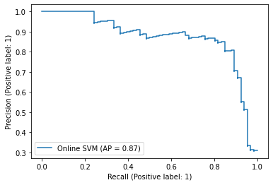
score_svm = pipe_svm.decision_function(test["tokens"])
PrecisionRecallDisplay.from_predictions(
    y_true=test["label_num"],
    y_pred=score_svm,
    name="Online SVM",
)
<sklearn.metrics._plot.precision_recall_curve.PrecisionRecallDisplay at 0x7fa4a5317370>
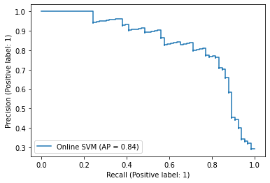
\(\alpha\) や、確率的勾配降下法のイテレーション数も変更できます。
scikit-learn のドキュメント Working With Text Data に出てくる設定で学習してみましょう。
pipe_svm = Pipeline([
    ("vect", TfidfVectorizer(tokenizer=str.split)),
    ("clf", SGDClassifier(loss="hinge", penalty="l2", alpha=1e-3, random_state=42, max_iter=5, tol=None)),
])
pipe_svm.fit(X=train["tokens"], y=train["label_num"])
Pipeline(steps=[('vect',
                 TfidfVectorizer(tokenizer=<method 'split' of 'str' objects>)),
                ('clf',
                 SGDClassifier(alpha=0.001, max_iter=5, random_state=42,
                               tol=None))])
In a Jupyter environment, please rerun this cell to show the HTML representation or trust the notebook. On GitHub, the HTML representation is unable to render, please try loading this page with nbviewer.org.
Pipeline(steps=[('vect',
                 TfidfVectorizer(tokenizer=<method 'split' of 'str' objects>)),
                ('clf',
                 SGDClassifier(alpha=0.001, max_iter=5, random_state=42,
tol=None))])TfidfVectorizer(tokenizer=<method 'split' of 'str' objects>)
SGDClassifier(alpha=0.001, max_iter=5, random_state=42, tol=None)
score_svm = pipe_svm.decision_function(test["tokens"])
PrecisionRecallDisplay.from_predictions(
    y_true=test["label_num"],
    y_pred=score_svm,
    name="Online SVM",
)
<sklearn.metrics._plot.precision_recall_curve.PrecisionRecallDisplay at 0x7fa4a13adf10>
ロジスティック回帰
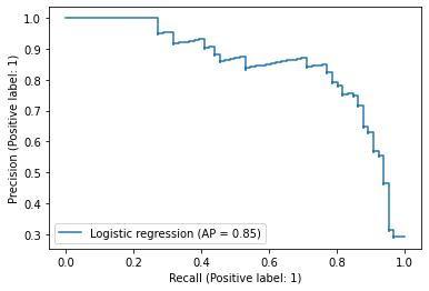
SGDClassifierで loss を log_loss にすることで、以下の目的関数を最適化するロジスティック回帰モデルに対応します。
学習してみましょう。
pipe_log = Pipeline([
    ("vect", TfidfVectorizer(tokenizer=str.split)),
    ("clf", SGDClassifier(loss="log_loss", random_state=0)),
])
pipe_log.fit(X=train["tokens"], y=train["label_num"])
Pipeline(steps=[('vect',
                 TfidfVectorizer(tokenizer=<method 'split' of 'str' objects>)),
                ('clf', SGDClassifier(loss='log_loss', random_state=0))])
In a Jupyter environment, please rerun this cell to show the HTML representation or trust the notebook. On GitHub, the HTML representation is unable to render, please try loading this page with nbviewer.org.
Pipeline(steps=[('vect',
                 TfidfVectorizer(tokenizer=<method 'split' of 'str' objects>)),
('clf', SGDClassifier(loss='log_loss', random_state=0))])TfidfVectorizer(tokenizer=<method 'split' of 'str' objects>)
SGDClassifier(loss='log_loss', random_state=0)
score_log = pipe_log.predict_proba(test["tokens"])[:,1]
PrecisionRecallDisplay.from_predictions(
    y_true=test["label_num"],
    y_pred=score_log,
    name="Logistic regression",
)
<sklearn.metrics._plot.precision_recall_curve.PrecisionRecallDisplay at 0x7fa4a5a43b20>
特徴量の重要度
SGDClassifierは線形分類器なので、特徴量の重みを見ることでその重要度を知ることができます。
特徴量の重みは coef_ で取得します。
coef = pipe_svm["clf"].coef_
coef.shape
(1, 3069)
特徴量のインデックスに対応するトークンを取得して、トークン毎の重要度を見てみましょう。
tokens = pipe_svm["vect"].get_feature_names_out()
tokens.shape
(3069,)
importance_df = pd.DataFrame({
    "importance": coef[0],
    "token": tokens,
})
ソートして重要度が高いものからいくつか表示してみましょう。
# ラベルが 1 (つまり意見がネガティブ)側の重要なトークン
importance_df.sort_values("importance", ascending=False).head(30)
| importance | token | |
|---|---|---|
| 2159 | 3.668755 | 残念 |
| 2353 | 2.423272 | 狭い |
| 1851 | 1.956964 | 悪い |
| 1696 | 1.739485 | 少し |
| 619 | 1.634807 | イマイチ |
| 1416 | 1.532445 | 古い |
| 335 | 1.509603 | ただ |
| 430 | 1.487909 | ない |
| 370 | 1.466131 | ちょっと |
| 2142 | 1.435011 | 欲しい |
| 452 | 1.329396 | ぬ |
| 1697 | 1.241647 | 少ない |
| 2194 | 1.191060 | 汚い |
| 198 | 1.133250 | が |
| 1949 | 1.130926 | 改善 |
| 2847 | 0.962159 | 遠い |
| 1667 | 0.909662 | 寒い |
| 138 | 0.890221 | いまいち |
| 3036 | 0.767494 | 髪の毛 |
| 547 | 0.762516 | もう |
| 2343 | 0.729504 | 物 |
| 632 | 0.718417 | エアコン |
| 289 | 0.692843 | すぎる |
| 2604 | 0.690301 | 臭い |
| 2317 | 0.676942 | 無い |
| 200 | 0.672533 | がっかり |
| 450 | 0.665977 | にくい |
| 1517 | 0.651460 | 壁 |
| 115 | 0.641441 | あまり |
| 153 | 0.627860 | うるさい |
# ラベルが 0 (つまり意見はポジティブ)側の重要なトークン
importance_df.sort_values("importance").head(30)
| importance | token | |
|---|---|---|
| 2612 | -0.955972 | 良い |
| 518 | -0.928854 | ます |
| 2563 | -0.644084 | 美味しい |
| 2052 | -0.631138 | 最高 |
| 958 | -0.594304 | ホテル |
| 2549 | -0.583404 | 綺麗 |
| 2374 | -0.552146 | 申し分 |
| 218 | -0.537186 | くれる |
| 119 | -0.530833 | ある |
| 2295 | -0.510448 | 満足 |
| 230 | -0.505866 | こと |
| 1618 | -0.501718 | 嬉しい |
| 1835 | -0.494761 | 快適 |
| 2029 | -0.486436 | 普通 |
| 1214 | -0.478245 | 便利 |
| 546 | -0.472399 | も |
| 2346 | -0.459666 | 特に |
| 1418 | -0.453142 | 可 |
| 1769 | -0.444798 | 広い |
| 130 | -0.441114 | いただく |
| 0 | -0.436411 | ! |
| 2789 | -0.414795 | 近い |
| 1332 | -0.413389 | 利用 |
| 283 | -0.411962 | しれる |
| 2519 | -0.407408 | 素晴らしい |
| 1362 | -0.397935 | 助かる |
| 2915 | -0.396517 | 間違い |
| 1164 | -0.394688 | 以上 |
| 394 | -0.393395 | で |
| 302 | -0.387782 | すむ |
単語を見ると意見のポジティブ、ネガティブを反映して特徴量である各トークンに重要度が与えられていることがわかります。